The CEO walks into the lab on Monday morning. Sales has a customer on the line who needs to commit to 50,000 plants of cultivar X delivered by the end of August. "Can we do it?" she asks. If your honest answer right now is "let me go look at the trays" — or worse, "yes, probably" — you're not actually forecasting; you're guessing.
The math to answer that question defensibly isn't exotic — any competent tissue culture manager has done it on paper at some point. The harder problem is that the forecast isn't a one-time question; it's an ongoing tracking task. You need it current to know whether each cultivar is on track for its committed ship-week, and to decide what to start more of, what to slow down, and what to reroute. Inventory drifts week to week as contamination happens, multiplication rates vary, and orders shift; a forecast that was right on Monday is often wrong by Friday. Most labs run it manually once a quarter (or once a year) and then trust it long after the inputs have moved underneath it, because re-running the whole order book by hand takes a day — and by the time anyone notices the answer has drifted, the inventory adjustments to fix it are already weeks late.
This is the methodology, worked end to end on real numbers. The math is the same whether a six-cultivar lab does it on paper or a thirty-cultivar lab runs it through software in seconds — but how often you can rerun it is what decides whether the answer is still worth anything by the time you act on it.
The five inputs every honest forecast depends on
A six-month forecast for any cultivar is a function of five things: the multiplication rate at each stage transition, the loss rate at each stage, the structure of your production network, the incubation time at each stage, and where your material is sitting right now. Get these five right and the rest is bookkeeping. Guess at any of them and the forecast lies.
| Input | What it captures | How you get it |
|---|---|---|
| Multiplication rate | Plants out per plant in at each stage transition, before losses are applied — the biological rate of the cultivar at that stage | Recorded counts at every subculture: containers consumed, plants produced on clean events, and which destination stage each child routed to |
| Loss rate | Fraction of plants lost between stages or during transitions — contamination, selection, and mortality. Combines with multiplication rate to give the effective rate the forecast realizes | Tagged discard events per stage, divided by throughput at that stage. Per cultivar; per season when the difference matters |
| Production network structure | The map of which stages feed which — the design of your pipeline plus the conditional routes lots actually take through it | Mapped from how your lab is set up to operate and what the routing data on recorded subcultures shows is happening |
| Incubation times | Calendar weeks a cultivar spends in each stage before being subcultured out | Measured from event-to-event intervals per stage, per cultivar — and per season when the difference matters |
| Current inventory | The launch position of the forecast — how much material is in each stage of the network right now, and how long it's been there | Counted from current lot records, or a bench audit when the records aren't current enough to trust |
Four of the five describe the network itself: its structure, the multiplication rate at each transition, the loss rate at each stage, and the incubation time at each stage. The fifth — current inventory — is the present state of the lab, the launching position from which the forecast is projecting forward. All five are directly readable from the event records the tissue culture lab records guide says belong on every work event; without those records, none of them are.
Why intuition fails six months out
Three reasons forecasts that "feel about right" are usually wrong by an order of magnitude:
Multiplication compounds
A multiplication rate of 6× over three subcultures isn't 18× — it's 216×. Over four subcultures: 1,296×. Eyeballing a "rough estimate" by adding stage outputs together undercounts by orders of magnitude. The math is exponential; intuition is linear.
The same exponential is why when you stop multiplying matters as much as that you can multiply at all. One multiplication cycle past your target gives you your multiplication rate × the inventory you actually needed — at a 6× rate, six times the plants the project committed to. Every one of those extra plants cost medium, jars, bench space, and tech time to produce, and the ones you can't sell come straight out of the project's margin. The most expensive failure mode here isn't a tech who can't subculture — it's a tech who runs one more cycle than the schedule needed because nobody noticed the target was already met. This is why running the forecast often enough matters so much: a forecast that's a week out of date doesn't just give you a wrong shipping number, it quietly lets you produce six times what you needed.
The same exponential is just as unforgiving in the other direction when your assumed rate is too high. A 0.5× gap between forecast and reality — say you planned for 3.0× per cycle but the cultivar is really doing 2.5× — is only a 17% shortfall after one subculture. Over six subcultures it becomes the difference between 729× and 244× starting-inventory growth: you arrive at production base with roughly a third of the plants you committed to ship, and no time left to multiply your way out of it. Even a 0.25× gap on a 3× rate compounds to a 40% shortfall over six cycles. This is why the multiplication rate in the forecast has to come from measured events for the specific cultivar, not a nominal number borrowed from elsewhere. A small cultivar-specific deviation, compounded across six subcultures, is the difference between hitting and missing a quarterly commitment.
Sub-1.0 rates also compound — and they're normal
A 0.6× per-output rate at a selection stage, repeated three times, is 0.216×: a 78% population collapse before the lot ever ships. Stages that split material across multiple destinations routinely produce per-output rates well below 1.0 — a single subculture that takes 153 source plants and splits them across three children at 1.41×, 0.53×, and 0.41× sums to a healthy 2.35× overall, but a forecast model that only tracks one destination per stage will compound the wrong sub-rate and underestimate (or overestimate) the destination it actually cared about. The fix is recording per-output rates on every event, not collapsing them into a single per-stage average.
Losses stack multiplicatively
A 5% loss at each of five stages isn't 5% total loss — it's
1 − (1 − 0.05)⁵ = 22.6%. Most spreadsheets model the
total as 5%. The difference compounds with multiplication: a nominal
6× rate combined with a 5% real loss rate gives a 5.7× effective
rate, but the same 6× combined with the true 22.6% cumulative loss
is closer to 4.6×. Over three subcultures the gap is 153× vs 97× —
the forecast is off by 35% from one bad assumption.
Eyeballing a rough estimate by adding stage outputs together undercounts by orders of magnitude. The math is exponential; intuition is linear.
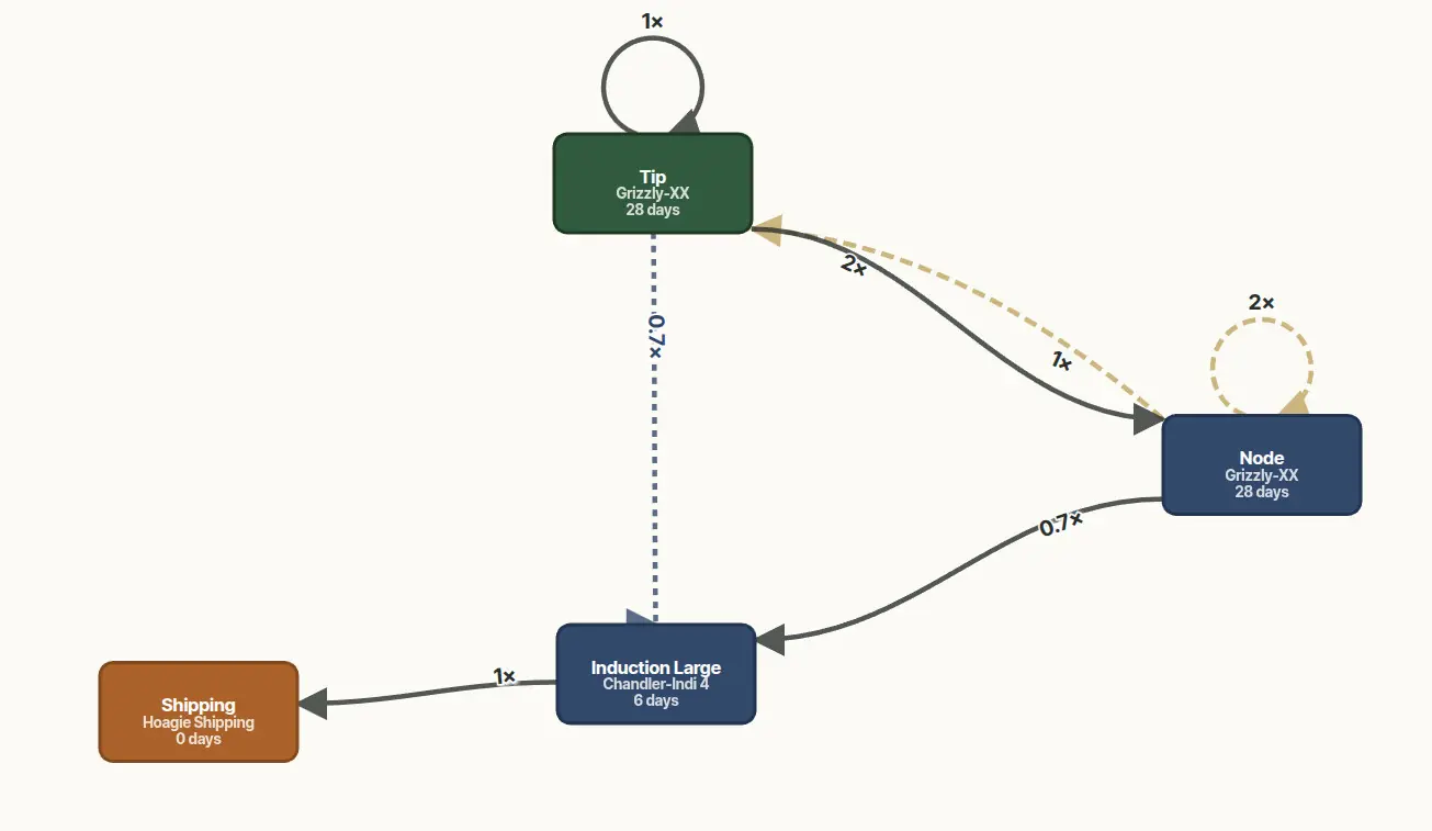
Production is a network, not a line
Most spreadsheet forecasts model production as a single chain — Multiplication → Induction → Rooting → Transitioning → Shipping — with one rate and one incubation time per stage. Real production isn't a chain. A single subculture event can produce multiple child lots that route to different destination stages, depending on what the source material looked like and what the downstream stages need. A typical multiplication-stage subculture might take 153 source plants and split them into three children — 216 plants advanced to Nodes for further multiplication, 81 plants moved to Transfer for capacity reasons, 63 plants prepared into Induction Large for rooting — at 1.41×, 0.53×, and 0.41× per output, summing to a healthy 2.35× overall for the event.
A production network is the map of how stages feed each other in your lab — the boxes and arrows in the figure above. Each box is a stage, each arrow is a transition between stages, and each arrow carries its own multiplication rate, loss rate, and incubation time. A forecast is what you get when you project current inventory forward through this map over time.
A forecast that only allows one transition out of each stage can't represent the splitting case at all. The result is a forecast that picks the wrong downstream rate to compound, and three months later the destination stage that "should have been ready" turns out to be undersupplied — usually because the routing pushed material somewhere else.
A worked example, six months out
Take cultivar X starting at 200 multiplication-stage plants on May 17, with a healthy network and disciplined records. Stage parameters:
| Transition | Incubation time | Multiplication rate | Loss rate |
|---|---|---|---|
| Multiplication → Multiplication (cycle) | 4 weeks | 6.0× | 5% |
| Multiplication → Induction | 4 weeks | 1.0× (no mult) | 5% |
| Induction → Rooting | 4 weeks | 1.0× | 8% |
| Rooting → Transitioning | 4 weeks | 1.0× | 10% |
| Transitioning → Shipping | 2 weeks | 1.0× | 0% |
Walked forward week by week (two multiplication cycles, then through root induction, rooting, transitioning, and into the shipping queue):
| Week | Stage | Population | Math |
|---|---|---|---|
| 0 | Multiplication | 200 | starting |
| 4 | Multiplication (cycle 1) | 1,140 | 200 × 6.0 × 0.95 |
| 8 | Multiplication (cycle 2) | 6,498 | 1,140 × 6.0 × 0.95 |
| 12 | Induction (entered) | 6,173 | 6,498 × 0.95 |
| 16 | Rooting (entered) | 5,679 | 6,173 × 0.92 |
| 20 | Transitioning (entered) | 5,111 | 5,679 × 0.90 |
| 22 | Shipping (available) | 5,111 | (transitioning complete) |
Twenty-two weeks — just over five months — from 200 multiplication-stage plants to ~5,100 shippable plants. To commit 50,000 plants by August you'd need either far more starting material, a third multiplication cycle (adding four weeks but pushing total available to ~29,000), or a fourth (another four weeks to ~166,000). One real-feeling cultivar, honestly modeled, gives the CEO a defensible answer instead of a shrug.
This is the kind of arithmetic any tech can do on paper for a single cultivar. The reason most labs don't is that one cultivar isn't the question — the question is the whole order book, against shared capacity, with conflicting due dates and contamination shocks arriving on Tuesday.
Where spreadsheets stop scaling
One cultivar, one network, six months out is a 20-row spreadsheet. The math doesn't change at scale; what changes is everything you have to layer on top of it:
- Shared capacity. Twenty cultivars competing for the same multiplication bench space. Each one's forecast depends on whether the others can fit alongside it.
- Stagger. Subculture cohorts ladder out over weeks. A "March multiplication cycle" is actually four cohorts started in different weeks of March, each ready at a slightly different time.
- Customer priorities. Orders have ship-week commitments. The same 5,000 plants ready in week 22 are worth very different things in week 18 versus week 26.
- Conditional routing. A subculture's destination depends on its quality, the downstream stage's current load, and what customer orders are still open.
At that point you're past what a spreadsheet can do by hand and into territory that needs a solver — software designed to find the best way to allocate limited resources across a lot of competing demands. The same kind of software schedules airline crews and routes delivery trucks. You give it the network, the rates and losses and incubation times, the bench-space limits, and the order book; it returns the best allocation. When something changes — a contamination event, a new order, a loss-rate update — it re-runs in seconds. The human job is to keep the inputs honest, not to re-do the math by hand every time something moves.
- One cultivar, single-chain network
- Rates assumed, not measured
- Sub-1.0 per-output rates flagged as errors
- Splits and conditional routes can't be represented
- Customer commitments live outside the model
- Recompute everything if one assumption changes
- Whole order book, full network
- Per-transition rates drawn from event records
- Per-output rates accepted as routing data
- Splits and conditional routing native to the model
- Customer ship-week commitments as constraints
- Re-solves in seconds for any assumption change
The three questions every quarterly forecast must answer
- What are we committed to ship? Customer orders plus contractual obligations plus internal targets, with ship-week dates attached. Forecasting in volume without dates is exercise without information.
- What is our actual bottleneck? It's almost always multiplication or rooting capacity. Almost never shipping. If a forecast says shipping is the bottleneck, the forecast has the wrong unit somewhere — usually containers being compared against plants.
- What's our loss-rate assumption, and is it from data? If the number in your forecast is "5% across the board," somebody made it up. Real loss rates are measured per stage, per cultivar, and where possible per season. A single universal number is the easiest place for the forecast to be wrong by 20%.
A worksheet for sketching your own
You can run this methodology on paper or in a spreadsheet today, tool-agnostic, before committing to anything:
- List your stages in order, with each transition as a separate line. If a stage routes to multiple destinations, each destination is its own line.
- For each transition: incubation time in weeks, multiplication rate (plants out per plant in), and loss rate (percent of plants lost). Pull from your own event records if you have them. Mark assumptions as assumptions if you don't.
- Starting population at each stage — count what's actually on the bench today, not what should be there.
- Apply transitions week by week for 26 weeks. The week-26 row of the shipping column is your honest six-month commitment.
- Vary one assumption at a time and recompute. The inputs that move the answer the most are the ones to measure first; the inputs that barely move it can stay as assumptions.
The exact math is identical whether you do it by hand, in Excel, or with a solver — what matters is that the assumptions are explicit, the network is mapped, and the numbers trace back to recorded events rather than someone's recollection. The CEO's "can we ship 50,000 by August?" then gets a one-sentence answer that ends with a number you can stake the quarter on: "Yes — if cultivar X starts a second multiplication cycle this week and we don't see a repeat of the May contamination," or "No — but 35,000 by August and the rest by mid-September if we shift the order from cultivar Y." Both answers are useful. The one you can't afford is "let me check the trays."